Compare means from baredSC results

baredSC outputs can be used to evaluate the fold-change of expression between 2 conditions.

Inputs

We use the same inputs as in previous input descriptions.

Run baredSC on each subpopulation

Let’s focus on cells of group 0.0 and group 3.0 (they correspond to each of the 2 gaussians found previously). To increase the speed we will use less bins (--nx 25):

$ for group in 0 3; do
    for nnorm in 1 2; do
      baredSC_1d \
        --input example/nih3t3_generated_2d_2.txt \
        --metadata1ColName 0.5_0_0_0.5_group \
        --metadata1Values ${group}.0 \
        --geneColName 0.5_0_0_0.5_x \
        --output example/first_example_1d_group${group}_${nnorm}gauss_25_neff200 \
        --nnorm ${nnorm} --nx 25 --minNeff 200 \
        --figure example/first_example_1d_group${group}_${nnorm}gauss_25_neff200.png \
        --title "first gene ${nnorm} gauss group${group} 25 bins neff200" \
        --logevidence example/first_example_1d_group${group}_${nnorm}gauss_25_neff200_logevid.txt
    done
    combineMultipleModels_1d \
      --input example/nih3t3_generated_2d_2.txt \
      --metadata1ColName 0.5_0_0_0.5_group \
      --metadata1Values ${group}.0 \
      --geneColName 0.5_0_0_0.5_x --nx 25 \
      --outputs example/first_example_1d_group${group}_1gauss_25_neff200 \
      example/first_example_1d_group${group}_2gauss_25_neff200 \
      --figure example/first_example_1d_group${group}_1-2gauss_25.png \
      --title "first gene group$group 25 bins 1 and 2 gauss"
  done

In one case, 100 000 samples were not sufficient.

We check the QC. We can now compare the results:

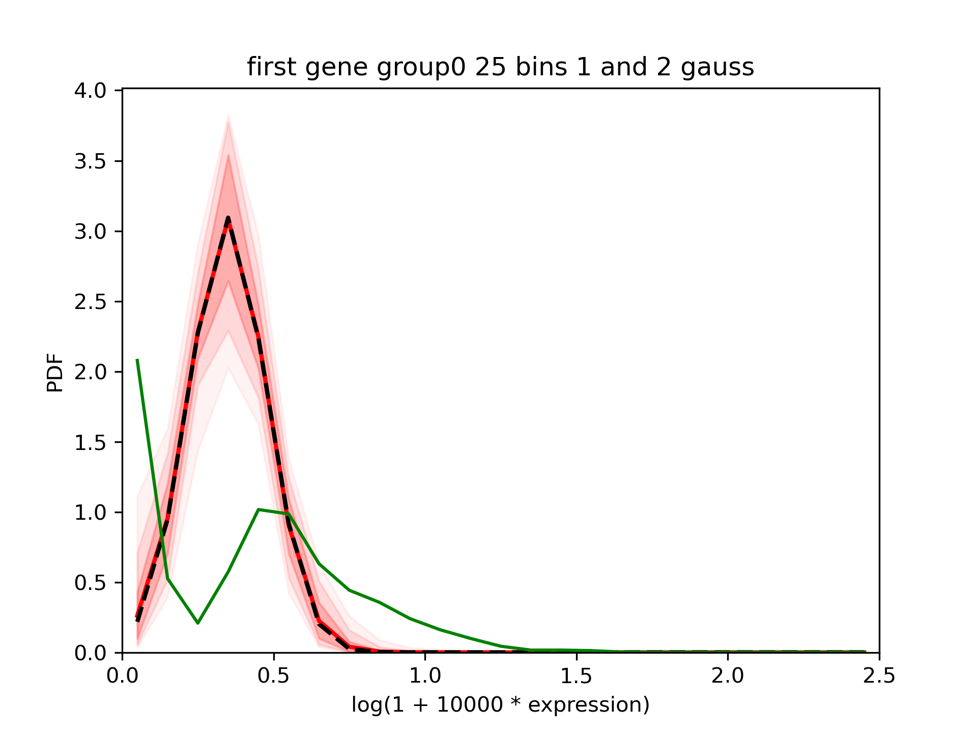
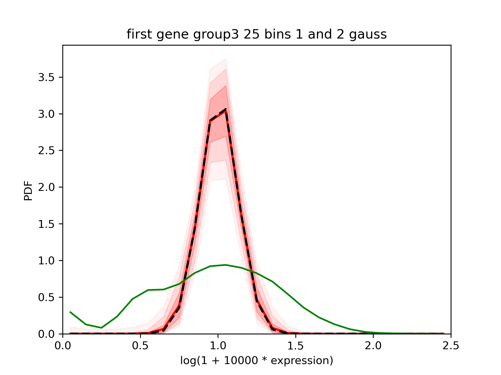
We can see that the tool fits relatively nicely the gaussians which were in inputs.

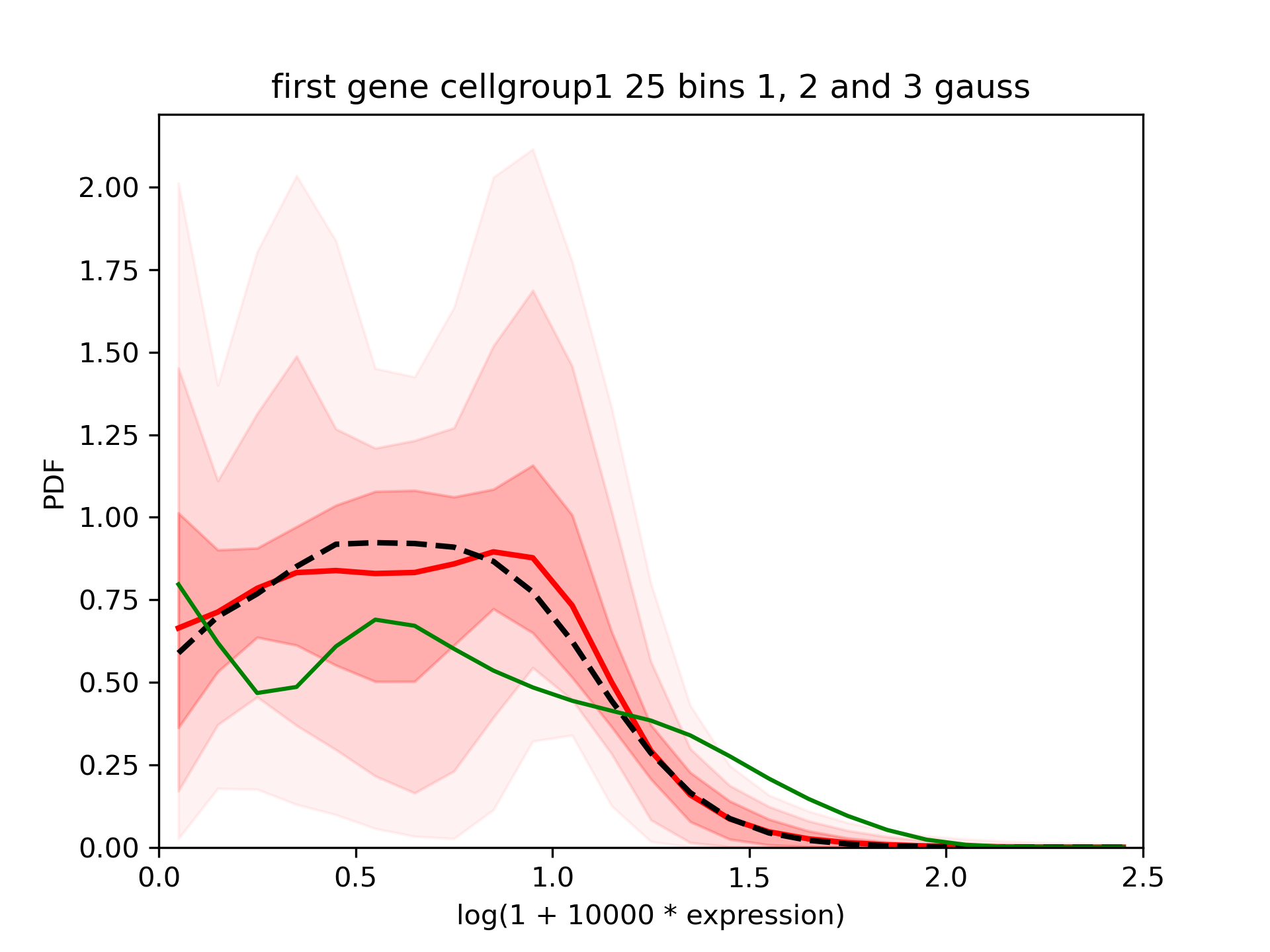
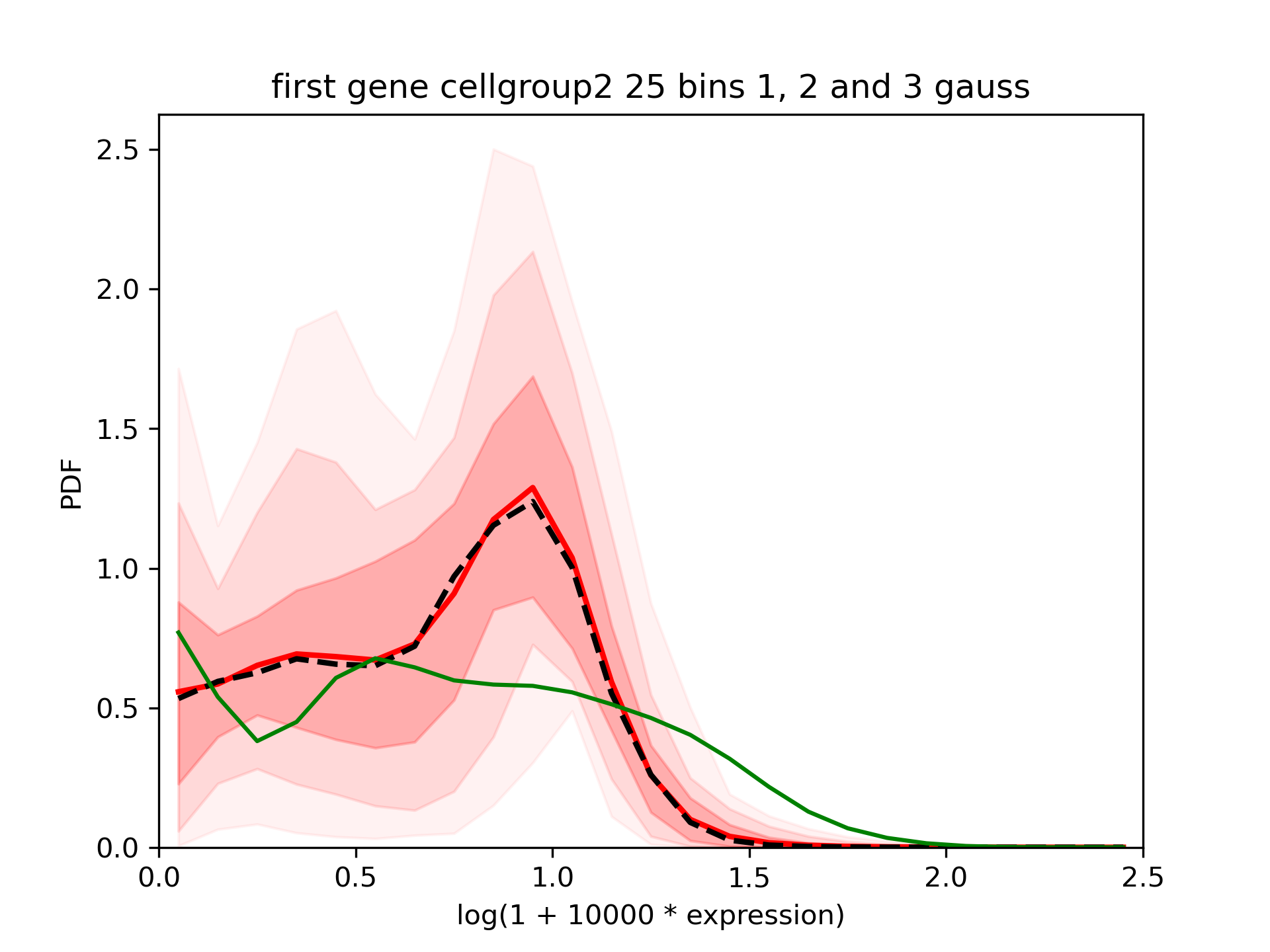
If we use another metadata which is just 300 and 500 random cells:

$ for group in 1 2; do
    for nnorm in 1 2 3; do
      baredSC_1d \
        --input example/nih3t3_generated_2d_2.txt \
        --metadata1ColName group \
        --metadata1Values group${group} \
        --geneColName 0.5_0_0_0.5_x \
        --output example/first_example_1d_cellgroup${group}_${nnorm}gauss_25_neff200 \
        --nnorm ${nnorm} --nx 25 --minNeff 200 \
        --figure example/first_example_1d_cellgroup${group}_${nnorm}gauss_25_neff200.png \
        --title "first gene ${nnorm} gauss cellgroup${group}" \
        --logevidence example/first_example_1d_cellgroup${group}_${nnorm}gauss_25_neff200_logevid.txt
    done
    combineMultipleModels_1d \
      --input example/nih3t3_generated_2d_2.txt \
      --metadata1ColName group \
      --metadata1Values group${group} \
      --geneColName 0.5_0_0_0.5_x --nx 25 \
      --outputs example/first_example_1d_cellgroup${group}_1gauss_25_neff200 \
      example/first_example_1d_cellgroup${group}_2gauss_25_neff200 \
      example/first_example_1d_cellgroup${group}_3gauss_25_neff200 \
      --figure example/first_example_1d_cellgroup${group}_1-3gauss_25.png \
      --title "first gene cellgroup$group 25 bins 1, 2 and 3 gauss"
  done

We see that the results are different in both groups but in both cases the confidence interval is quite large:

One of the output is *_means.txt.gz. Each line correspond to the value of the mean expression evaluated at each sample of the MCMC. It can be used to estimate:

• A confidence interval on the mean value (in the used axis log(1 + 10^4 * expression))

• A confidence interval on the fold change (delogged).

In [1]: import numpy as np
   ...: def delog(x):
   ...:     return(1e-4 * (np.exp(x) - 1))
   ...: my_quantiles = [0.5 - 0.6827 / 2, 0.5, 0.5 + 0.6827 / 2]
   ...: # Get data
   ...: means1 = np.genfromtxt('../example/first_example_1d_group0_1-2gauss_25_means.txt.gz')
   ...: print(f'Values of mean in group0: {means1}')
   ...: means2 = np.genfromtxt('../example/first_example_1d_group3_1-2gauss_25_means.txt.gz')
   ...: print(f'Values of mean in group3: {means2}')
   ...: # Shuffle means2
   ...: np.random.shuffle(means2)
   ...: print(f'Mean log expression in group0: {np.quantile(means1, my_quantiles)}')
   ...: print(f'Mean log expression in group3: {np.quantile(means2, my_quantiles)}')
   ...: fc = [delog(x1) / delog(x2) for x1, x2 in zip(means1, means2)]
   ...: print(f'Estimation of fold-change: {np.quantile(fc,  my_quantiles)}')
   ...: 
Values of mean in group0: [0.35776993 0.35776993 0.35776993 ... 0.34672964 0.34672964 0.38877004]
Values of mean in group3: [1.00746002 1.02085388 1.02085388 ... 1.00369734 1.01363153 1.02256951]
Mean log expression in group0: [0.33838793 0.34953488 0.36060358]
Mean log expression in group3: [0.99479228 1.00628287 1.01751424]
Estimation of fold-change: [0.23110761 0.24112418 0.25130651]

We can use matplotlib to display the results graphically:

In [2]: import matplotlib.pyplot as plt
   ...: x1, x2 = np.random.normal(1, 0.1, len(means1)), np.random.normal(3, 0.1, len(means2))
   ...: fig, axs = plt.subplots(1, 2)
   ...: axs[0].scatter(x1, means1, s=1, alpha=0.01)
   ...: axs[0].scatter(x2, means2, s=1, alpha=0.01)
   ...: axs[0].set_ylim(0, )
   ...: axs[0].set_ylabel('log(1 + expression * 10\'000)')
   ...: axs[0].set_xticks([1, 3])
   ...: axs[0].set_xticklabels(['group0', 'group3'], fontsize='x-large')
   ...: axs[1].scatter(x1[:len(fc)], fc, s=1, alpha=0.01)
   ...: axs[1].set_xticks([1])
   ...: axs[1].set_xticklabels(['fold-change'], fontsize='x-large')
   ...: axs[1].set_ylim(0, )
   ...: axs[1].set_ylabel('Fold-change (not log transformed)')
   ...: fig.tight_layout()
   ...: 

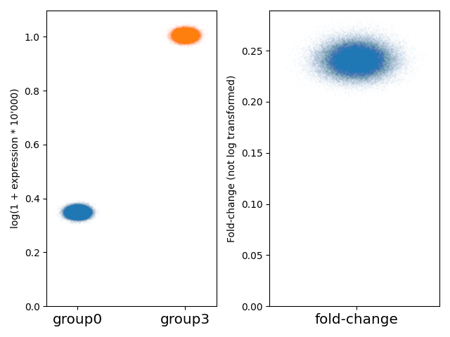
On the first example with group0 and group3 where each is a different gaussian, we see a mean log expression around the expected 0.375 value in group 0, 1 in group 3. We see that the fold-change is around 25% (this is the real fold-change, not log transformed).

Now if we have a look to the subsamples of cells (300 and 500 cells) and perform the same analysis:

In [3]: # Get data
   ...: means1 = np.genfromtxt('../example/first_example_1d_cellgroup1_1-3gauss_25_means.txt.gz')
   ...: print(f'Values of mean in cellgroup1: {means1}')
   ...: means2 = np.genfromtxt('../example/first_example_1d_cellgroup2_1-3gauss_25_means.txt.gz')
   ...: print(f'Values of mean in cellgroup2: {means2}')
   ...: # Shuffle means2
   ...: np.random.shuffle(means2)
   ...: print(f'Mean log expression in cellgroup1: {np.quantile(means1, my_quantiles)}')
   ...: print(f'Mean log expression in cellgroup2: {np.quantile(means2, my_quantiles)}')
   ...: fc = [delog(x1) / delog(x2) for x1, x2 in zip(means1, means2)]
   ...: print(f'Estimation of fold-change: {np.quantile(fc,  my_quantiles)}')
   ...: 
Values of mean in cellgroup1: [0.66035127 0.66035127 0.62547552 ... 0.62783495 0.62783495 0.62783495]
Values of mean in cellgroup2: [0.68203872 0.69214061 0.71198453 ... 0.70698152 0.70698152 0.70698152]
Mean log expression in cellgroup1: [0.6161945  0.64620379 0.67630369]
Mean log expression in cellgroup2: [0.66763529 0.69110072 0.71426981]
Estimation of fold-change: [0.8423754  0.91214824 0.9865969 ]

In [4]: x1, x2 = np.random.normal(1, 0.1, len(means1)), np.random.normal(3, 0.1, len(means2))
   ...: fig, axs = plt.subplots(1, 2)
   ...: axs[0].scatter(x1, means1, s=1, alpha=0.01)
   ...: axs[0].scatter(x2, means2, s=1, alpha=0.01)
   ...: axs[0].set_ylim(0, )
   ...: axs[0].set_ylabel('log(1 + expression * 10\'000)')
   ...: axs[0].set_xticks([1, 3])
   ...: axs[0].set_xticklabels(['cellgroup1', 'cellgroup2'], fontsize='x-large')
   ...: axs[1].scatter(x1[:len(fc)], fc, s=1, alpha=0.01)
   ...: axs[1].set_xticks([1])
   ...: axs[1].set_xticklabels(['fold-change'], fontsize='x-large')
   ...: axs[1].set_ylim(0, )
   ...: axs[1].set_ylabel('Fold-change (not log transformed)')
   ...: fig.tight_layout()
   ...: 

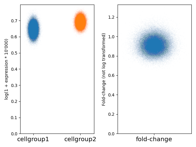
Here, we can see that the fold-change is slightly below 1.